Oil & Gas — Volumes & Economics
From a prospect to a P90 reserve estimate, EUR, expected value and an AFE cost range — all as distributions, not point estimates
Five models for the subsurface and the money that follows it. Unlike the rest of Flexa Analytics these are parameter-driven: you do not drop a table into the visual. You describe each input as a distribution in the form and the simulation does the rest, which is what you want when the well has not been drilled yet and there is no history to sample.
Answer the question: "Every number in this AFE is an estimate with a range behind it. What does the range of outcomes actually look like, and which input is driving it?"
The five models on this page
| Model | What it computes | Key inputs |
|---|---|---|
| Reserves (P10/P50/P90) | Volumetric oil-in-place and recoverable reserves from rock and fluid uncertainty | Area · Thickness · Porosity · Sw · NTG · Bo · RF |
| Project Economics (NPV/IRR) | Cash-flow model over a production profile — NPV, IRR, payback, breakeven price | Price · Capex · Opex · Production profile · Discount |
| Decline Curve (EUR) | Arps decline to estimated ultimate recovery | Initial rate qi · Decline Di · Arps b · Horizon |
| Exploration EMV | Expected monetary value of a prospect — chance of success against dry-hole cost | NPV if success · Dry-hole cost · Probability of success |
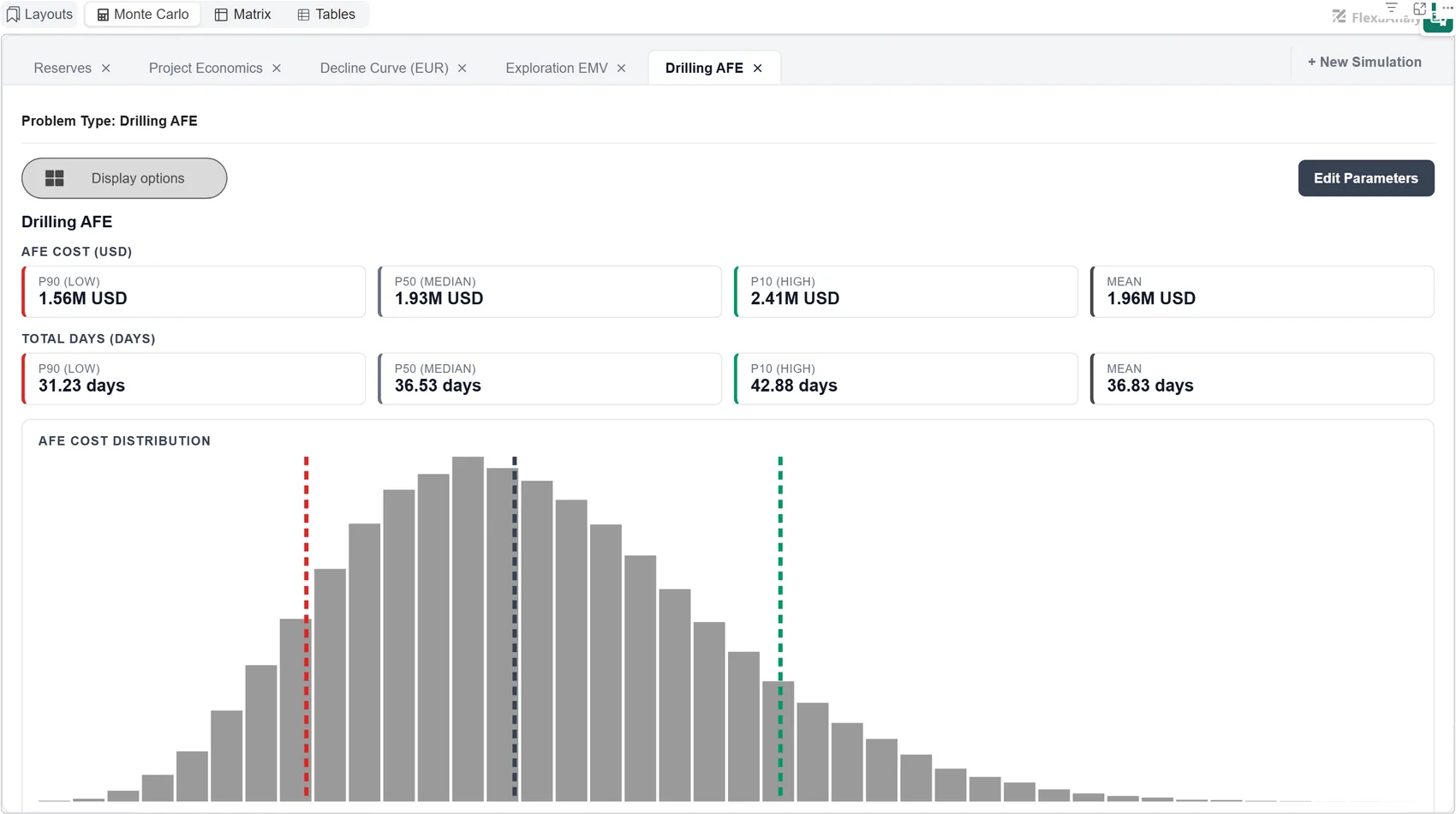
| Drilling AFE | Well cost from planned days, day rate and non-productive time | Planned days · Day rate · NPT days · Flat cost |
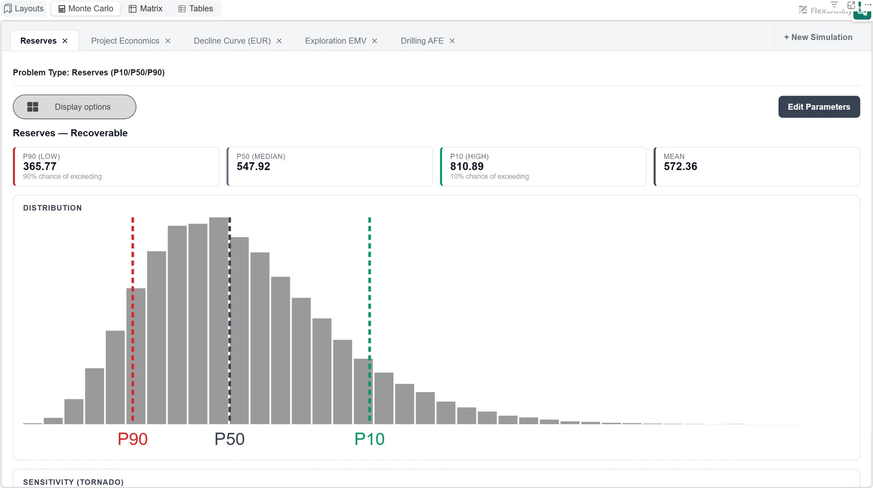
Reserves (P10/P50/P90)
The classic volumetric calculation, run ten thousand times. Each of the seven rock and fluid properties is a distribution rather than a single number, so the output is a reserves range instead of a figure that pretends the subsurface is known.
Default parameters:
- ▸Area:PERT(400, 500, 650)
- ▸Thickness (gross pay):PERT(20, 30, 45)
- ▸Porosity:Triangular(0.15, 0.20, 0.28)
- ▸Water saturation:Uniform(0.20, 0.40)
- ▸Net-to-Gross:Uniform(0.70, 1.0)
- ▸FVF (Bo):Uniform(1.1, 1.3)
- ▸Recovery factor:PERT(0.20, 0.35, 0.50)
Project Economics (NPV/IRR)
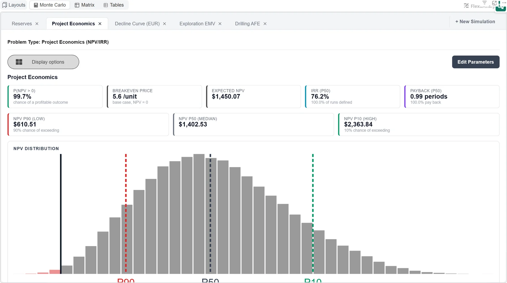
Takes a production profile and prices it. Reports the probability the project makes money at all, the breakeven price that puts NPV at zero, and the NPV range — the three numbers an investment committee actually asks for.
Default parameters:
- ▸Price:Triangular(6, 10, 16)
- ▸Capex:PERT(800, 1000, 1300)
- ▸Opex fixed:Triangular(60, 100, 140)
- ▸Opex variable (per unit):Uniform(0.5, 1.5)
- ▸Production multiplier:PERT(0.7, 1.0, 1.2)
- ▸Production profile:120, 100, 80, 60
- ▸Discount / Escalation / Royalty / Tax:0.10 / 0 / 0 / 0
Decline Curve (EUR)
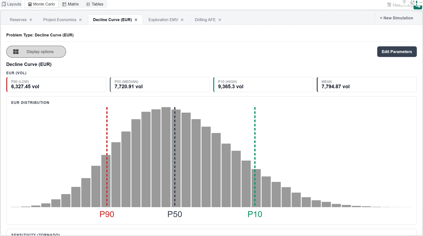
Projects a well forward from its initial rate using Arps decline, with the b exponent as a distribution. That last part matters: b decides whether the tail is exponential or hyperbolic, and it is where most of the disagreement about EUR lives.
Default parameters:
- ▸Initial rate (qi):PERT(800, 1000, 1400)
- ▸Decline (Di):Triangular(0.08, 0.12, 0.20)
- ▸Arps b:Triangular(0, 0.5, 1) — hyperbolic: (1.0, 1.5, 2.0)
- ▸Horizon:15 periods
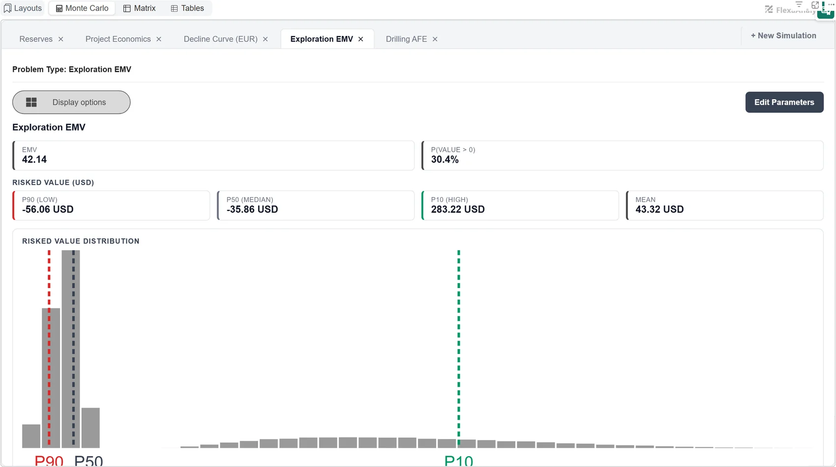
Exploration EMV
The drill-or-drop calculation. Weighs the value if the well works against the cost if it does not, and reports both the expected value and the probability the outcome is positive at all.
Default parameters:
- ▸NPV if success:PERT(50, 200, 600)
- ▸Dry-hole cost:PERT(20, 40, 80)
- ▸Probability of success:0.30
Drilling AFE
An AFE that admits trouble happens. Non-productive time is its own distribution rather than a flat contingency percentage, so the cost range reflects how bad a stuck pipe or a weather window actually gets.
Default parameters:
- ▸Planned days:PERT(25, 30, 45)
- ▸Day rate:Triangular(40000, 50000, 70000)
- ▸NPT days:PERT(0, 4, 15)