
How to Convert Row to Column in Power BI
1. Why Convert Rows to Columns in Power BI?
Converting rows to columns — pivoting — reorganizes data into a more readable cross-tab format. A dataset with monthly sales stored as rows becomes a table where months are column headers and products are rows, making period-over-period comparison immediate.
The three most common reasons to pivot in Power BI:
2. Method 1: Flexa Tables — Pivot at the Visual Layer
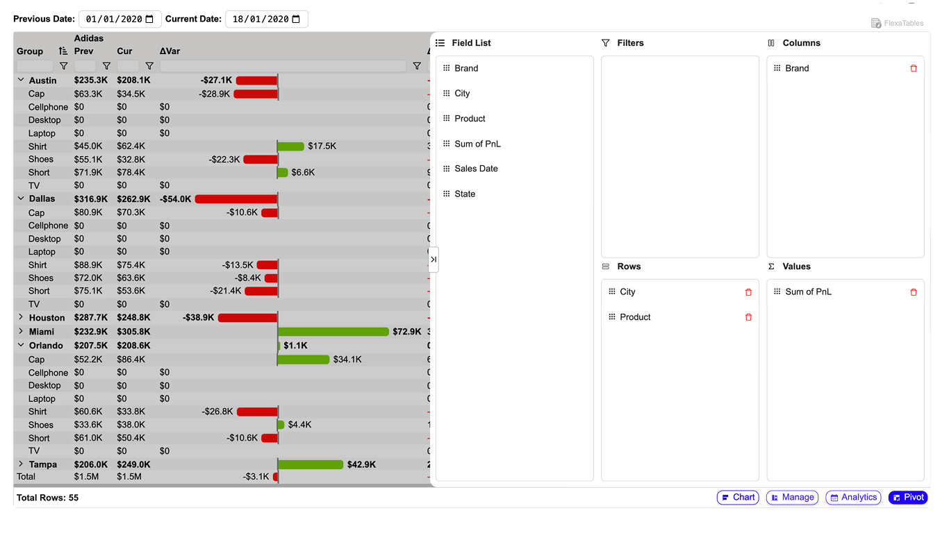
Flexa Tables is a Microsoft-certified custom visual from AppSource that adds true drag-and-drop pivot behavior to Power BI — the behavior that Excel pivot tables have but Power BI's native Matrix visual doesn't. The key difference: Flexa Tables lets end users restructure rows and columns after publishing, in Power BI Service, without going back to Desktop.
Step 1: Import your data
- Open Power BI Desktop.
- Home → Get Data → Excel → select your file → Load.
- Verify in Data View: columns like Date, Product, Sales are present.
Step 2: Add Flexa Tables to your report
- Insert → More Visuals → AppSource → search "Flexa Tables" → Add.
- Drag the Flexa Tables visual onto your report canvas.
- Resize to full width for best readability.
Step 3: Configure the pivot
- Rows: Drag Product to the Rows field — products appear as row headers.
- Columns: Drag Date (Year-Month) to the Columns field — months become column headers.
- Values: Drag Sales to the Values field — cells show aggregated sales per product per month.
- Publish to Power BI Service — end users can now drag fields to restructure the pivot themselves.
3. Method 2: Power Query Pivot Column
Power Query Pivot Column reshapes your data at the model level — before it reaches any visual. Use this when your source data arrives in tall format (one row per period) and a downstream system or specific report layout requires a fixed wide table.
- Home → Transform Data to open Power Query Editor.
- Select the column whose values will become column headers (e.g. the Month column).
- Transform → Pivot Column.
- In the dialog, select the Values Column (e.g. Sales). Set Aggregate to Sum.
- Click OK — Power Query creates one column per unique value in the selected field.
- Home → Close & Apply.
Works with any downstream visual
No self-service after publishing
4. Method 3: DAX + Matrix Visual
The native Matrix visual pivots data at the visual layer — no Power Query transformation needed. Place your row dimension in Rows, your column dimension (Month, Quarter, Scenario) in Columns, and your measure in Values. The Matrix generates a cross-tab layout at render time.
-- Basic measure to use in the Matrix Values field
Total Sales = SUM(Sales[Sales])
Drag Product to Rows, Date (Year-Month) to Columns, and Total Sales to Values. The Matrix handles the pivot at render time — no data model changes needed.
5. Which Method Should You Use?
6. Enhancing Pivoted Data with Variance Analysis
Once your data is in cross-tab format, the next step for Finance and analytics teams is usually variance analysis — comparing each cell against a budget, prior year, or prior period.
With native Power BI, variance columns require separate DAX measures that multiply as your metrics grow. With Flexa Tables, users add MoM, YoY, Actual vs Budget, and Actual vs Forecast columns directly in the Analytics panel in the published report — no DAX, no Desktop round trip.
7. Best Practices and Common Errors
Best practices
- Clean before pivoting: Remove blank rows and duplicate identifier combinations in Power Query before applying any pivot step.
- Keep column count reasonable: More than 20 columns in a cross-tab hurts readability. Use a date slicer to limit the visible range.
- Default to tall format in the data model: Power BI's DAX time intelligence functions are designed for normalized (tall) data. Only pivot at the visual layer unless a specific downstream requirement forces otherwise.
- Validate: After pivoting, cross-check totals against your source data to catch silent aggregation errors.
Common errors
IF(ISBLANK([Total Sales]), 0, [Total Sales]) to show zero instead.


