Executive Summary: Global Oil Production Analysis (1960–2024)
793 Downloads
Description
1. Key Insights (Data Analysis)
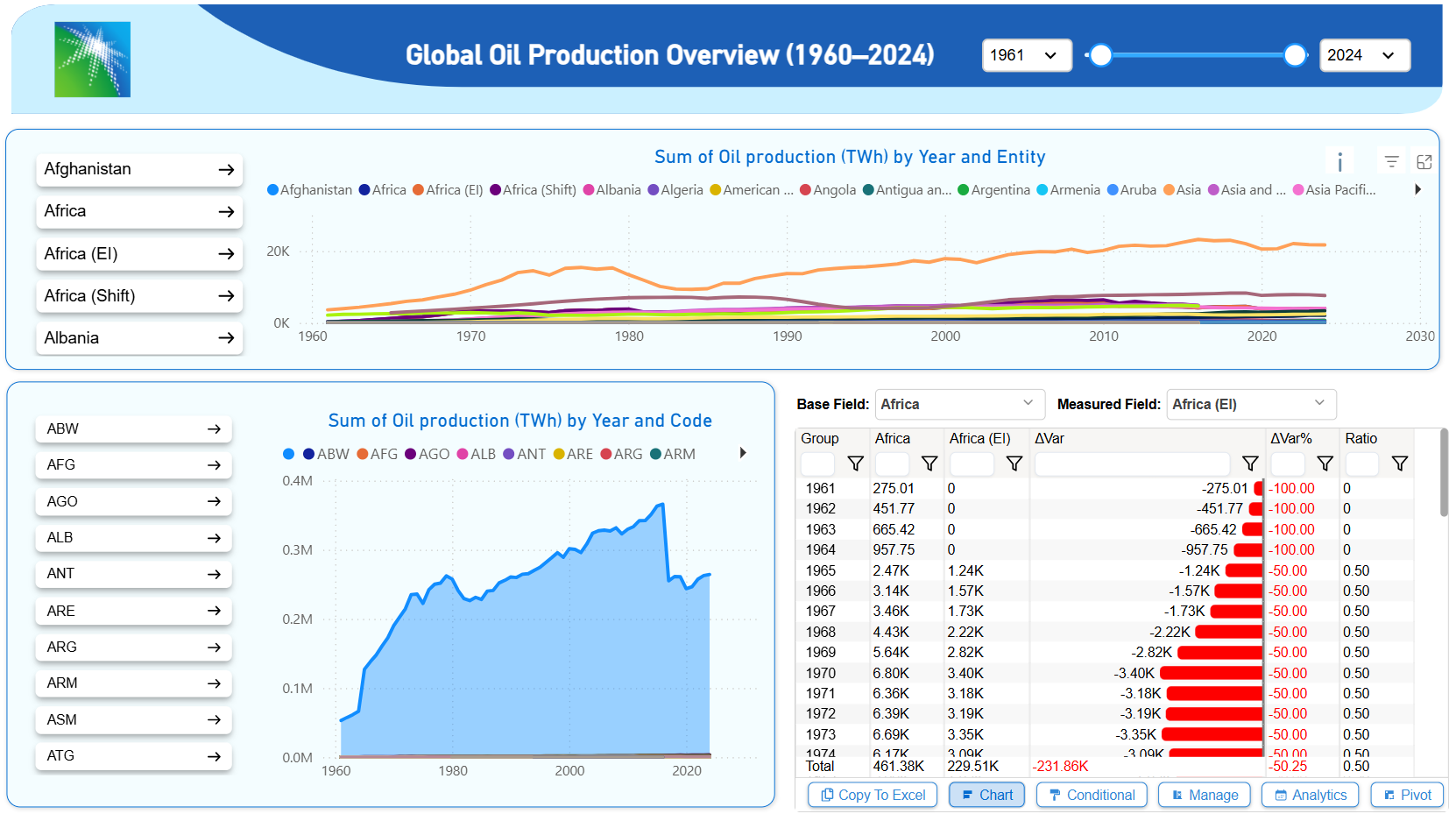
- Long-term Production Trends: * The Line Chart shows a steady upward trajectory in global production since the 1960s, with a noticeable peak around the late 1970s followed by a period of volatility.
- The Area Chart reveals a significant production dip around 2020, likely corresponding to the global impact of the COVID-19 pandemic, followed by a volatile recovery phase.
- Regional Performance Discrepancies:
- The detailed table focuses on a comparison between Africa and Africa (EI).
- There is a consistent -50.25% variance in the total measured field. From 1965 onwards, the "Measured Field" (Africa EI) is consistently exactly half of the "Base Field" (Africa), resulting in a fixed Ratio of 0.50.
- Data Anomalies:
- In the early years (1961–1964), the variance was -100%, indicating missing data or a lack of reporting from the "Africa (EI)" entity during that period.
2. Technical Insights (Dashboard Design)
- Effective Visual Hierarchy: The dashboard uses a clear structure with global filters at the top and specific country/code slicers on the left, allowing for easy navigation.
- Advanced Table Functionality: The use of Flexa Tables (or similar advanced grids) is evident. The conditional formatting (red data bars for $\Delta Var\%$) successfully draws the eye to negative variances, making it easy to spot underperformance or data gaps.
- Time-Series Granularity: The inclusion of both a line chart (for multi-entity comparison) and an area chart (for volume distribution) provides a dual-layer understanding of the data.
3. Strategic Recommendations
For Data & Analytics:
- Investigate the 0.50 Ratio: The fact that the ratio is exactly 0.50 for decades suggests either a specific mathematical definition (e.g., one field measuring crude only while the other measures total liquids) or a potential calculation error in the data transformation layer.
- Data Completion: Address the -100% variance between 1961 and 1964. If historical data is unavailable, it should be noted in a tooltip or a footnote to avoid misinterpretation of "zero production."
For Dashboard Enhancement:
- Incorporate a Sankey Diagram: Since you are interested in flow visualization, adding a Sankey Diagram would be excellent for showing how total global production "flows" into different regions or usage types (e.g., Export vs. Domestic Consumption).
- Dynamic Forecasting: Add a "Forecast" line to the line chart using Power BI’s native analytics features to project production trends toward 2030 based on historical patterns.
- Optimize Sidebar Space: The left-hand slicer list is quite long. Consider using a "Dropdown" or a "Searchable Slicer" to save screen real estate for larger visualizations.
Other Templates
 Free Supply Chain & Logistics
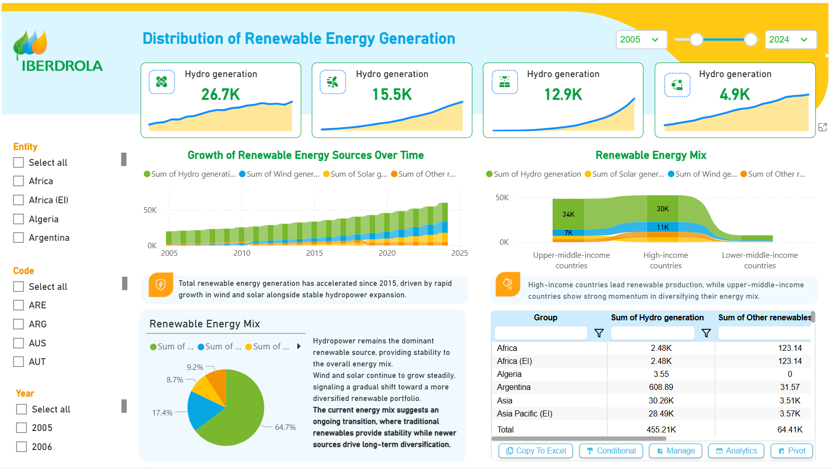
IBERDROLA Distribution of Renewable Energy Generation Dashboard – Key Insights (2005–2024)
968
 Free Sales & Revenue
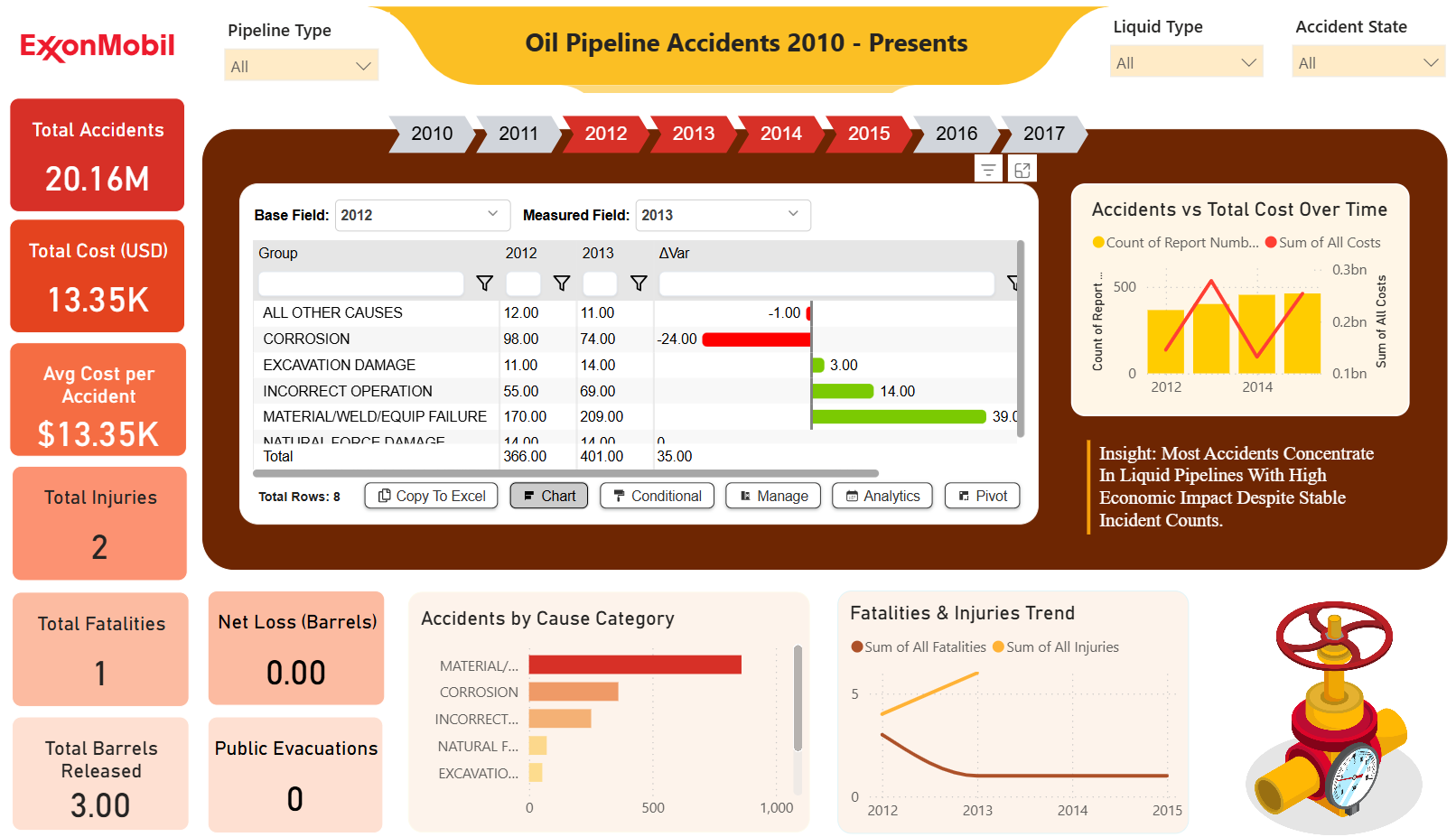
ExxonMobil Oil Pipeline Accidents Dashboard (2010–Present) – Key Insights
921
 Free Sales & Revenue
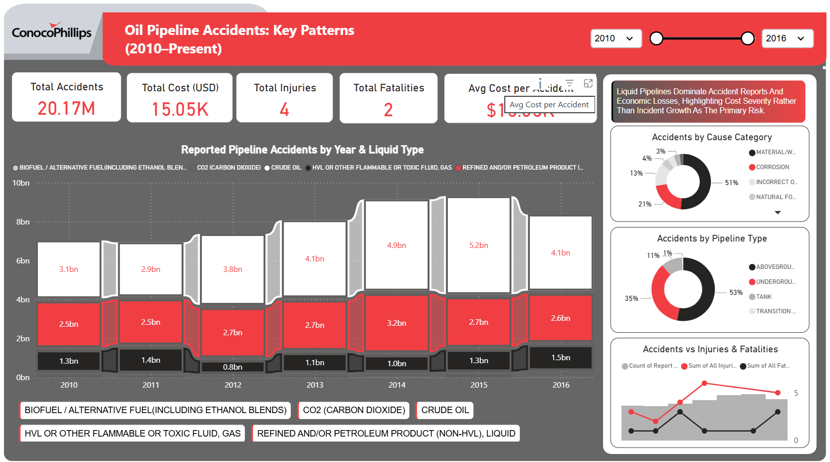
ConocoPhillips Oil Pipeline Accidents: Key Patterns (2010–Present) – Key Insights
871
If you find this website helpful, share it with friends and colleagues to boost their Power BI skills and work efficiency!
Like this site? Share it